Mapping in the Complex Plane

The mapping of functions in the complex plane is conceptually simple, but will lead us to a very powerful technique for determining system stability. In addition it will give us insight into how to avoid instability. To introduce the concept we will start with some simple examples. There are several videos on this page - they merely support the written material, but are not absolutely vital.

Mapping of Functions with a Single Zero

The simplest functions to map are those with a single zero. Several examples follow.

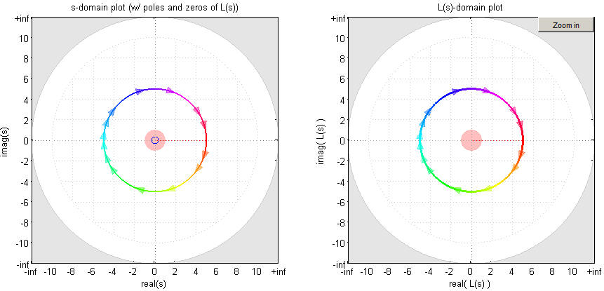
Example: Mapping with circle in "s", zero at the origin in "L(s)"

Consider the trivial function L(s)=s (we will deal with more complicated functions later, this simple function allows us to introduce concepts associated with mapping). We let the variable s traverse a circular path centered at the origin with a radius of 5 moving in the clockwise direction (the left side graph), In other words

We then plot L(s) on the right hand graph. This is shown in the image below, followed soon thereafter by a video that better demonstrates the mapping.

Notes about image above

There are several aspects about the image above that are important (many of these come up later):

The path in the "s" plane is shown at the left. It is a circle of radius 5, centered at the origin and moving in a clockwise direction, as indicated by the arrows.
The arrows show the direction of motion, but the spacing of the arrows is arbitrary.
The colors of the two plots match, so that the portion of "s" that is yellow is also yellow on "L(s)". This is obvious here, but becomes a useful distinction in more complex plots to come.
There is a pink circle centered on the zero in the "s" plane. This shows the angle subtended between the zero and the path in s. You can see the growth of this circle (in the clockwise direction) in the video below.
There is also a pink circle centered on the origin in the "L(s)" plane. This shows the angle subtended between the origin and the path in s. The color indicates the direction; pink indicates the clockwise direction. If the direction had been counterclockwise it would be blue.
Note that as the path in "s" encircles the zero one time in the counterclockwise direction, the path in "L(s)" encircles the origin once in the same direction.

Example: Mapping with circle in "s", zero at s=-4

If we now place a zero at s=-4 so that L(s)=s+4, the mapping is still very straightforward. Every location in "s" simply maps to a location that is 4 units to the right in "L(s)". The path in s remains as before. (Note: this example is also considered as part of the video above.)

Notes about image above

The path in "s" is still a circle, as is the path in "L(s)", but the path is simply offset by 4 (since L(s)=s+4.
Note that as the path in "s" encircles the zero one time in the clockwise direction, the path in "L(s)" encircles the origin once in the same direction.
As the path in "s" gets near the pole in "L(s)" (where the path has a light blue color), the path in "L(s)" becomes the smallest (i.e., the closest to the origin). This is because the term in the numerator, in this case (s+4), is minimal when "s" is near the pole at -4. Also, when the distance from the zero to the path in "s" is maximal (red), so is the distance from L(s) to the origin.

Example: Mapping with circle in "s", zero at s=-6

If we now place a zero at s=-6 so that L(s)=s+6, the mapping is still very straightforward. Every location in "s" simply maps to a location that is 4 units to the right in "L(s)." The path in s remains as before. (Note: this example is also considered as part of the video above.)

Notes about image above

The path in "s" is still a circle, as is the path in "L(s)", but the path is simply offset by 4 (since L(s)=s+4.
Note that as the path in "s" no longer encircles the zero, and the path in "L(s)" no longer encircles the origin.

Comments about mapping with a zero in "L(s)"

There are three important, and general, statements we can now make about mapping from "s" to "L(s)" when there is a zero in "L(s)":

Mapping with a single pole

Mapping of functions with a single pole is not much more difficult than mapping with a single zero. There are two important facts about encirclements of poles that can be shown by considering L(s) with a single pole at the origin, and the path in "s" being a clockwise circle of radius 'r' around the origin:

The mapping around various functions, L(s), with a single poles are shown in the diagrams in the examples below, followed by a video that shows several functions. Each example in the video is also included in the examples that follow. It is useful to read the examples before viewing the video.

Example: Mapping with circle in "s", pole at origin

If we choose L(s) such that it has a pole at the origin,

(note: the constant multiplier makes the plots looks nicer, but isn't necessary for the mathematics to work)

and we let s follow the same path as before

We get

Because the e^jθwas originally in the denominator, its sign is changed when it moves to the numerator. In other words, the path in "L(s)" is a circle of radius 2 that encircles the origin once in the clockwise direction.

Notes about image above

The path in the "s" plane is shown at the left. It is a circle of radius 5, centered at the origin and moving in a clockwise direction.
There is a blue circle centered on the pole in the "s" plane (a pink circle will be used for zeros, as in the previous angles). This shows the angle subtended between the pole and the path in s. You can see the growth of this circle in the video below.
There is a grey circle centered on the origin in the "L(s)" plane. This shows the angle subtended between the origin and the path in s.
Note that as the path in "s" encircles the pole one time in the clockwise direction, the path in "L(s)" encircles the origin once in the opposite (counterclockwise) direction.

Example: Mapping with circle in "s", pole at s=-4

If we now place a pole at s=-4 so that

Note: this example is also considered as part of the video above.)

The path in s remains as before, but the path in "L(s)" has changed. The center and extent of the path in "L(s)" have both changed.

(note: if you can show that the path in "L(s)" is also a circle and derive equations for the radius and center, I'll include it here, with an acknowledgement for the first person who sent it to me)

Notes about image above

The path in "s" still encircles the pole in a clockwise direction, and the path in "L(s)" still encircles the origin in a counterclockwise (opposite) direction.
As the path in "s" gets near the pole in "L(s)" (where the path has a light blue color), the path in "L(s)" becomes the largest (i.e., the farthest from the origin). This is because the term in the denominator, in this case (s+4), is minimal when "s" is near the pole at -4. Also, when the distance from the pole to the path in "s" is maximal (red), the distance from L(s) to the origin is minimal

Example: Mapping with circle in "s", pole at s=-6

If we now place a pole at s=-6 so that

Note: this example is also considered as part of the video above.)

The path in s remains as before, but the path in "L(s)" has changed. The center and extent of the path in "L(s)" have both changed.

Notes about image above

Note that as the path in "s" no longer encircles the pole in a clockwise direction, and the path in "L(s)" no longer encircles the origin.

Example: Mapping with circle in "s", pole at s=-4.8

If we now place a pole at s=-4.8 so that

Note: this example is also considered as part of the video above.)

The path in s remains as before, but the path in "L(s)" has changed. The center and extent of the path in "L(s)" have both changed. The shape

(note: if you can show that the path in "L(s)" is also a circle and derive equations for the radius and center, I'll include it here, with an acknowledgement for the first one to send it to me)

Notes about image above

Note that as the path in "s" encircles the pole in a clockwise direction, and the path in "L(s)" still encircles the origin in a counterclockwise direction.
As the path in "s" comes very close to the pole in "L(s)" (where the paths are light blue), the path in "L(s)" becomes very large. In these diagrams this is shown as going towards infinity. In these plots, anything with a radius of more than twelve is truncated and shown at infinity.

Comments about mapping with a pole in "L(s)"

There are thee important, and general, statements we can now make about mapping from "s" to "L(s)" when there is a pole in "L(s)":

Mapping with multiple poles and/or zeros

If you understand the concept of mapping of functions with individual poles and zeros, it is not much harder to understand mapping of functions with multiple poles and zeros. A few examples will illustrate this. You should read through the first example carefully, it has a lot of important information.

Example: L(s) has two poles, one zero; all are encircled

Consider mapping of the transfer function

where s follows a clockwise circular path of radius 5 around the origin , as before.

To get an idea of what the mapping will look like, let's express the function in polar notation.

At this point we are mostly interested in the angle of L(s), so lets examine it more closely.

Recall that, in general, the angle

is determined by drawing a line from s₀ to s, and finding the angle between that line and the horizontal (described here). So if we let s₀=-2, then the angle

would be determined by drawing a line from s=-2 to s and finding the angle to the horizontal. This is shown in the diagram below on the left for angles between the location s=-5j to the zero at -2, and the poles at -1 and -3.

Since the angle of L(s) is given by

then this is the angle shown in the image above on the right. Since we know the first term in the angle of L(s) goes from 0→-2*π, and we subtract the other two terms, then the angle of L(s) must go from 0→2*π, that is it encircles the origin once in the counterclockwise direction. This can be seen in the image below, and in the video that follows.

Notes about image above

The path in "s" encircles the poles and zero in the clockwise direction.
The angle between the path and the zero is shown in red, and the angle between the path and the pole is shown in blue. The path in "L(s)", which is shown in gray, is the sum of the angles from the zeros (red) minus the angles from the poles (blue). This is more obvious in the video.
If a path in "s" encircles Z zeros and P poles of L(s) in the clockwise direction, then the path in "L(s)" encircles the origin N=Z-P times in the clockwise direction. In this case Z=1, P=2 so N=-1, and we have one encirclement of the origin in "L(s)" in the counterclockwise direction.

Aside: Magnitude of L(s)

The magnitude of L(s) is given by

This means that if s is very close to a zero (i.e., near s=-2) that the magnitude of L(s) becomes very small, and if s is very close to a pole (i.e., near s=-1 or s=-3) that the magnitude of L(s) becomes very large.

Example: L(s) has two poles, one zero, one pole; one zero is encircled

Now if we change the transfer function to

then the path in s encircles the zero, but only one of the poles.

Notes about image above

If a path in "s" encircles Z zeros and P poles of L(s) in the clockwise direction, then the path in "L(s)" encircles the origin N=Z-P times in the clockwise direction. In this case Z=1, P=1 so N=0, and we have no encirclements of the origin in "L(s)".

Example: L(s) has two poles, one zero; one zero is encircled

Now if

then the path in "s" encircles only the zero

Notes about image above

If a path in "s" encircles Z zeros and P poles of L(s) in the clockwise direction, then the path in "L(s)" encircles the origin N=Z-P times in the clockwise direction. In this case Z=1, P=0 so N=1, and we have one encirclement of the origin in "L(s)" in the clockwise direction.

Example: L(s) has two poles, one zero; two poles are encircled

Now if

then the path in "s" encircles only the zero

Notes about image above

If a path in "s" encircles Z zeros and P poles of L(s) in the clockwise direction, then the path in "L(s)" encircles the origin N=Z-P times in the clockwise direction. In this case Z=0, P=2 so N=-2, and we have two encirclements of the origin in "L(s)" in the clockwise direction.
You can tell there are two encirclements because the circle in "L(s)" is twice as dark. This is more clear in the video.

Example: L(s) has two complex conjugate poles encircled by s

Consider

Poles at -2±4j which are inside a circle with radius 5.

Notes about image above

If a path in "s" encircles Z zeros and P poles of L(s) in the clockwise direction, then the path in "L(s)" encircles the origin N=Z-P times in the clockwise direction. In this case Z=0, P=2 so N=-2, and we have two encirclements of the origin in "L(s)" in the clockwise direction.

Example: L(s) has two complex conjugate poles not encircled by s

Consider

Poles at -4±4j, which are outside a circle of radius 5.

Notes about image above

If a path in "s" encircles Z zeros and P poles of L(s) in the clockwise direction, then the path in "L(s)" encircles the origin N=Z-P times in the clockwise direction. In this case Z=0, P=0 so N=0 and we have no encirclements of the origin in "L(s)".

Video: Mapping with a multiple poles and zeros
(3½ minute video created with the Matlab script NyquistGui)

The path in "s" need not be circular

Nothing that we have done so far depends on the fact that the path in "s" be circular, which is important to the development of the Nyquist stability criterion on the next web page. Two examples below (and a video) demonstrate this. In the first example, immediately below, the path in "s" encircles a zero in the clockwise direction, and the path in "L(s)" encircles the origin in the same direction. In this first example L(s)=s, i.e., there is a zero at the origin.

In the second example, below, the path in "s" encircles a pole in the clockwise direction, and the path in "L(s)" encircles the origin in the opposite direction, Though the path is a very different shape. Note also that where the distance from the path in "s" to the pole is minimal (i.e., where the path is light blue), then the distance of path in "L(s)" to the origin is maximal (and where the distance in "s" is maximal (where the path is red), the distance in "L(s)" is minimal). In this example L(s)=10/(s+6), i.e., there is a pole at s=-6.

Video: Mapping with a multiple poles and zeros
(2 minute video created with the Matlab script NyquistGui))

Key Concept: Mapping from "s" to "L(s)"

The key points to keep in mind as you move to the next page:

If a path in "s" encircles a zero of L(s) in the clockwise direction, then this contributes 360° in the clockwise direction to the path in "L(s)" as it moves around the origin.
If a path in "s" encircles a pole of L(s) in the clockwise direction, then this contributes 360° in the counter clockwise direction to the path in "L(s)" as it moves around the origin.
If a path in "s" encircles Z zeros and P poles of L(s) in the clockwise direction, then the path in "L(s)" encircles the origin N=Z-P times in the clockwise direction. If N is negative, this corresponds to encirclements in the counterclockwise direction.
The path in "s" need not be circular.

Moving Forward

After reading through the material above, the question arises "So what?". What we have done here is introduce a technique that gives use information about the number of poles and zeros in a closed contour. To determine the stability of a system, we want to determine if a system's transfer function has any of poles in the right half plane. With just a little more work, we can define our contour in "s" as the entire right half plane - then we can use this to determine if there are any poles in the right half plane.

Mapping in the Complex Plane